Behind the Scenes

Basic concepts

GaussPy is a Python implementation of the AGD algorithm described in Lindner et al. (2015), AJ, 149, 138. At its core, AGD is a fast, automatic, extremely versatile way of providing initial guesses for fitting Gaussian components to a function of the form \(f(x) + n(x)\), where \(n(x)\) is a term modeling possible contributions from noise. It is important to emphasize here that although we use terminology coming from radio-astronomy all the ideas upon which the code is founded can be applied to any function of this form, moreover, non-Gaussian components can also be in principle extracted with our methodology, something we will include in a future release of the code.

Ideally, if blending of components was not an issue and \(n(x)=0\) the task of fitting Gaussians to a given spectrum would be reduced to find local maxima of \(f(x)\). However, both of these assumptions dramatically fail in practical applications, where blending of lines is an unavoidable issue and noise is intrinsic to the process of data acquisition. In that case, looking for solutions of \({\rm d}f(x)/{\rm d}x = 0\) is not longer a viable route to find local extrema of \(f(x)\), instead a different approach must be taken.

AGD uses the fact that a local maximum in \(f(x)\) is also a local minimum in the curvature. That is, the algorithm looks for points \(x^*\) for which the following conditions are satisfied.

• The function \(f(x)\) has a non-trivial value

\[f(x^*) > \epsilon_0.\]

In an ideal situation where the contribution from noise vanishes we can take \(\epsilon_0=0\). However, when random fluctuations are added to the target function, this condition needs to be modified accordingly. A good selection of \(\epsilon_0\) thus needs to be in proportion to the RMS of the analyzed signal.

• Next we require that the function \(f(x)\) has a “bump” in \(x^*\)

\[\left.\frac{{\rm d}^2f}{{\rm d}x^2}\right|_{x=x^*} < 0,\]

this selection of the inequality ensures also that such feature has negative curvature, or equivalently, that the point \(x^*\) is candidate for being the position of a local maximum of \(f(x)\). Note however that this is not a sufficient condition, we also need to ensure that the curvature has a minimum at this location.

• This is achieved by imposing two additional constraints on \(f(x)\)

\[\left.\frac{{\rm d}^3f}{{\rm d}x^3}\right|_{x=x^*} = 0\]

\[\left.\frac{{\rm d}^4f}{{\rm d}x^4}\right|_{x=x^*} > 0\]

These 4 constraints then ensure that the point \(x^*\) is a local minimum of the curvature. Furthermore, even in the presence of both blending and noise, these expressions will yield the location of all the points that are possible candidates for the positions of Gaussian components in the target function. The following is an example of a function defined as the sum of three gaussians for which the above conditions are satisfied and the local minima of curvature are successfully found, even when blending of components is relevant.

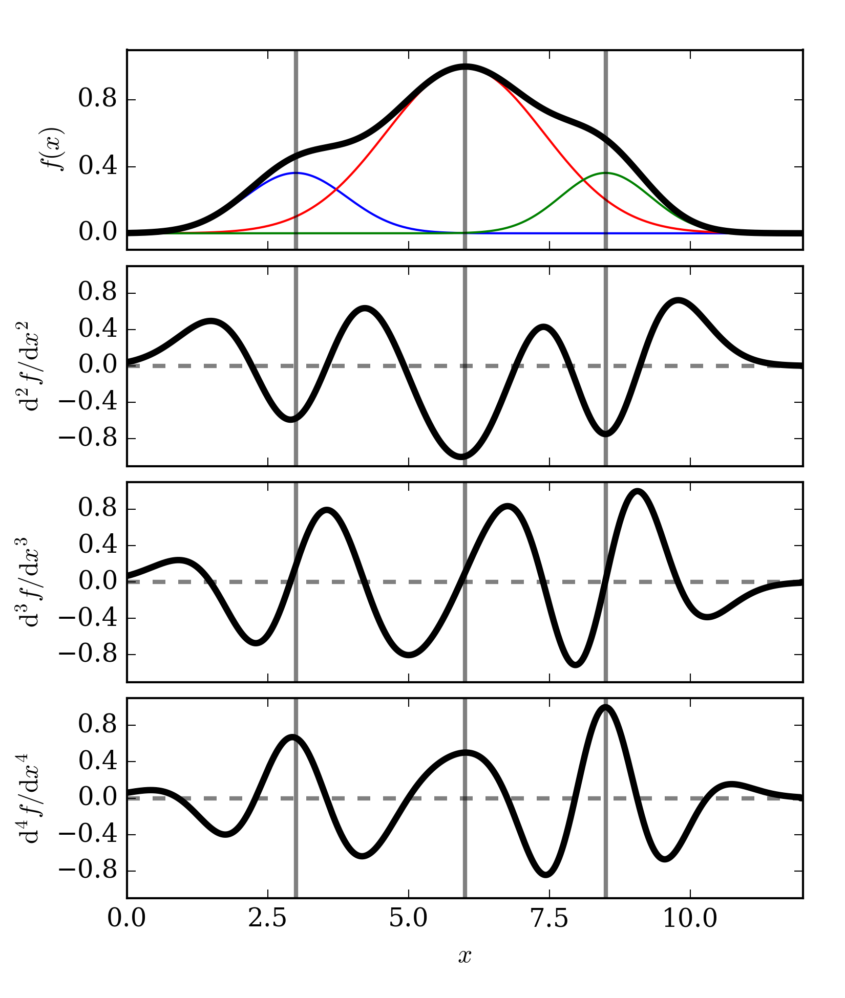
Example of the points of negative curvature of the function \(f(x)\). In this case \(f(x)\) is the sum of three independent Gaussian functions (top). The vertical lines in each panel show the conditions imposed on the derivatives to define the points \(x^*\).

Dealing with noise

The numeral problem related to the solution shown in the previous section comes from the fact that calculating derivatives is not trivial in the presence of noise. For instance, if the top panel of our example figure is sampled with 100 channels, and in each panel a random uncorrelated noise component is added at the 10% level, a simple finite difference prescription to calculate the derivative would lead to variations of the order \(\sim 1 / {\rm d}x \sim 10\). That is, the signal would be buried within the noise!

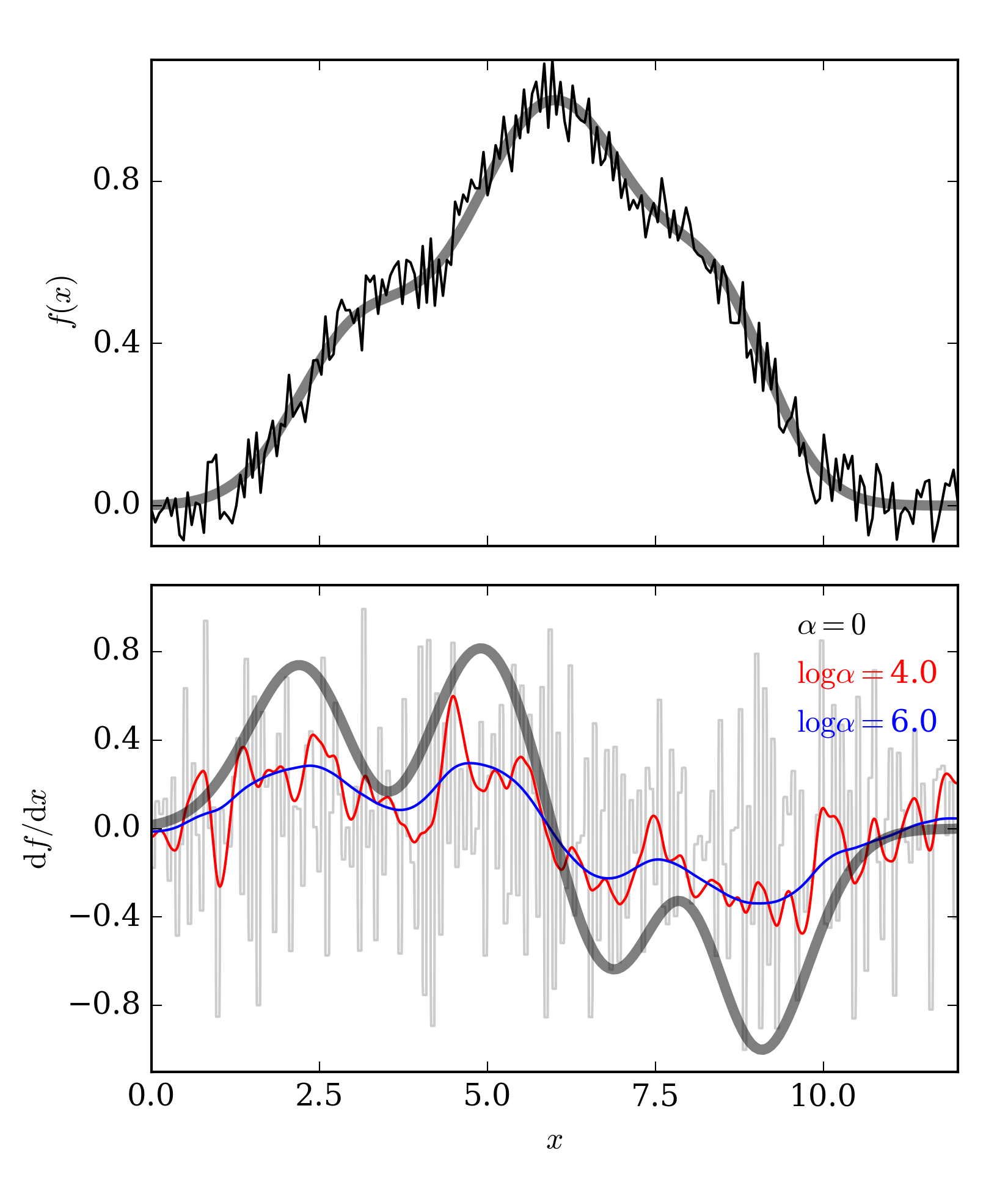
The top panel shows the same function used in the first example figure, but now random noise has been added to each channel. In the bottom panel we show various estimates of the first derivative. \(\alpha=0\) corresponds to the finite differences method, larger values of \(\alpha\) makes the function smoother.

In order to solve this problem AGD uses a regularized version of the derivative (Vogel (2002)). If \(u = {\rm d}f(x)/{\rm d}x\), then the problem we solve is \(u = {\rm arg}\min_u\{R[u]\}\) where \(R[u]\) is the functional defined by

\[R[u] = \int | A u - f | + \alpha \int \sqrt{(Du)^2 + \beta^2},\]

where \(A u = \int {\rm d}x\; u\). Note that if \(\alpha=0\) this is equivalent to find the derivative of the function \(f(x)\), since we will be minimizing the difference between the integral of \(u = {\rm d}f(x)/{\rm d}x\) and \(f(x)\) itself. This, however, has the problem we discussed in the previous paragraph. It is clear that this simple approach fails to recover the behavior of the target function. If, on the other hand, \(\alpha > 0\), an additional weight is added to the inverse problem in the equation for \(R[u]\), and now the differences between successive points in \(u(x)\) are taken into account.

The parameter \(\alpha\) then controls how smooth the derivative is going to be. The risk here is that overshooting the value of this number can erase the intrinsic variations of the actual derivative. What is the optimal value of \(\alpha\)? This question is answered by GaussPy through the training process of the algorithm. We refer the reader to the example chapters to learn how to use this feature.

Two phases

Within GaussPy is built-in the ability to automatically choose the best value of \(\alpha\) for any input data set. Special caution has to be taken here. If a component is too narrow it can be confused with noise and smoothed away by the algorithm!

In order to circumvent this issue GaussPy can be trainend in “two-steps”. One for narrow components, and one for broad components. The result then is two independent values \(\alpha_1\) and \(\alpha_2\) each giving information about the scales of different features in the target function.

An alternative approach

There is another alternative for calculating derivatives of noise-ridden data, namely convolving the function with a low-pass filter kernel, e.g., a Gaussian filter. Although the size of the filter can be optimized by using a training routine, in a similar fashion as we did for the \(\alpha\) scales, this technique is much more agressive and could lead to losses of important features in the signal. Indeed, the total variation scheme that GaussPy uses could be thought of as the first order approximation in a perturbative expansion of a Gaussian filter.

Notwhistanding this caveat GaussPy implements also a Gaussian filter as an option for taking the numerical derivatives. In total, there are three selectable modes within the package for calculating \(f(x) + n(x)\)

• GaussianDecomposer.set('mode','python'): This will execute GaussPy with a Python implementation of the total variation algorithm. The code is clean to read, easy to understand and modify, but it may perform slow for large datasets.

• GaussianDecomposer.set('mode','conv'): When this mode is set, the function is Gaussian-filtered prior to calculating the numerical derivative. In this case, the constant \(\alpha\) is taken to be the size of the kernel

  (1)\[\tilde{f}(x) = (f \star K_\alpha)(x) \quad\mbox{with}\quad K_\alpha(x) = \frac{1}{\sqrt{2\pi \alpha^2}}{\rm e}^{-x^2/2\alpha^2}.\]

  Once this mode is selected the training for choosing the optimal size of the filter proceeds in the same way we have discussed in the previous sections, i.e., nothing else has to be changed.