Prepping a Datacube¶

In this example we will download a datacube to decompose into individual spectra. The example cube we will use is from the GALFA-HI emission survey at the Arecibo Observatory, specifically the GALFA-HI M33 datacube from Putman et al. 2009. You can directly download the cube from here:

http://www.astro.columbia.edu/~mputman/M33only.fits.gz

Storing Data cube in GaussPy-Friendly Format¶

Before decomposing the datacube, we must store the data in a format readable by GaussPy. The following code provides an example of how to read a fits-formatted datacube and store the spectral information. The necessary parameters to specify here are:

FILENAME_DATA: the fits filename of the target data cube
FILENAME_DATA_GAUSSPY: the filename to store the GaussPy-friendly data in
RMS: estimate of the RMS uncertainty per channel for constructing the error arrays

# Read fits datacube and save in GaussPy format
import numpy as np
import pickle
from astropy.io import fits

# Specify necessary parameters
FILENAME_DATA = 'M33only.fits'
FILENAME_DATA_GAUSSPY = 'cube.pickle'
RMS = 0.06

hdu_list = fits.open(FILENAME_DATA)
hdu = hdu_list[0]
cube = hdu.data

# initialize
data = {}
errors = np.ones(cube.shape[0]) * RMS
chan = np.arange(cube.shape[0])

# cycle through each spectrum
for i in xrange(cube.shape[1]):
    for j in xrange(cube.shape[2]):

        # get the spectrum
        spectrum = cube[:, i, j]

        # get the spectrum location
        location = np.array((i, j))

        # Enter results into GaussPy-friendly dataset
        data['data_list'] = data.get('data_list', []) + [spectrum]
        data['x_values'] = data.get('x_values', []) + [chan]
        data['errors'] = data.get('errors', []) + [errors]
        data['location'] = data.get('location', []) + [location]

# Save decomposition information
pickle.dump(data, open(FILENAME_DATA_GAUSSPY, 'w'))

The output pickle file from the above example code contains a python dictionary with four keys, including the independent and dependent arrays (i.e. channels and spectral values), an array per spectrum describing the uncertainty per channel, and the (x,y) pixel location within the datacube for reference.

Creating a Synthetic Training Dataset¶

Before decomposing the target dataset, we need to train the AGD algorithm to select the best values of \(\log\alpha\) in two-phase decomposition. First, we construct a synthetic training dataset composed of Gaussian components with parameters sampled randomly from ranges that represent the data as closely as possible.

RMS: root mean square uncertainty per channel
NCHANNELS: number of channels per spectrum
NSPECTRA: number of spectra to include in the training dataset
NCOMPS_lims: range in total number of components to include in each spectrum
AMP_lims, FWHM_lims, MEAN_lims: range of possible Gaussian component values, amplitudes, FWHM and means, from which to build the spectra
TRAINING_SET : True or False, determines whether the decomposition “answers” are stored along with the data for accuracy verification in training
FILENAME_TRAIN : filename for storing the training data

# Create training dataset with Gaussian profile
import numpy as np
import pickle

def gaussian(amp, fwhm, mean):
    return lambda x: amp * np.exp(-4. * np.log(2) * (x-mean)**2 / fwhm**2)

# Estimate of the root-mean-square uncertainty per channel (RMS)
RMS = 0.06

# Specify the number of spectral channels (NCHANNELS)
NCHANNELS = 680

# Specify the number of spectra (NSPECTRA)
NSPECTRA = 200

# Estimate the number of components
NCOMPS_lims = [3,6]

# Specify the min-max range of possible properties of the Gaussian function paramters:
AMP_lims = [0.5,30]
FWHM_lims = [20,150] # channels
MEAN_lims = [400,600] # channels

# Indicate whether the data created here will be used as a training set
# (a.k.a. decide to store the "true" answers or not at the end)
TRAINING_SET = True

# Specify the pickle file to store the results in
FILENAME_TRAIN = 'cube_training_data.pickle'

# Initialize
data = {}
chan = np.arange(NCHANNELS)
errors = np.ones(NCHANNELS) * RMS

# Begin populating data
for i in range(NSPECTRA):
    spectrum_i = np.random.randn(NCHANNELS) * RMS

    amps = []
    fwhms = []
    means = []

    ncomps = np.random.choice((np.arange(NCOMPS_lims[0],NCOMPS_lims[1]+1)))

    for comp in xrange(ncomps):
        # Select random values for components within specified ranges
        a = np.random.uniform(AMP_lims[0], AMP_lims[1])
        w = np.random.uniform(FWHM_lims[0], FWHM_lims[1])
        m = np.random.uniform(MEAN_lims[0], MEAN_lims[1])

        # Add Gaussian profile with the above random parameters to the spectrum
        spectrum_i += gaussian(a, w, m)(chan)

        # Append the parameters to initialized lists for storing
        amps.append(a)
        fwhms.append(w)
        means.append(m)

    # Enter results into AGD dataset
    data['data_list'] = data.get('data_list', []) + [spectrum_i]
    data['x_values'] = data.get('x_values', []) + [chan]
    data['errors'] = data.get('errors', []) + [errors]

    # If training data, keep answers
    if TRAINING_SET:
        data['amplitudes'] = data.get('amplitudes', []) + [amps]
        data['fwhms'] = data.get('fwhms', []) + [fwhms]
        data['means'] = data.get('means', []) + [means]

# Dump synthetic data into specified filename
pickle.dump(data, open(FILENAME_TRAIN, 'w'))

Training AGD to Select \(\alpha\) values¶

With a synthetic training dataset in hand, we train AGD to select two values of \(\log\alpha\) for the two-phase decomposition, \(\log\alpha_1\) and \(\log\alpha_2\). The necessary parameters to specify are:

FILENAME_TRAIN: the pickle file containing the training dataset in GaussPy format
snr_thresh: the signal to noise ratio below which GaussPy will not fit a component
alpha1_initial, alpha2_initial initial choices of the two \(\log\alpha\) parameters

# Train AGD using synthetic dataset
import numpy as np
import pickle
import gausspy.gp as gp
reload(gp)

# Set necessary parameters
FILENAME_TRAIN = 'cube_training_data.pickle'
snr_thresh = 5.
alpha1_initial = 4
alpha2_initial = 12

g = gp.GaussianDecomposer()

# Next, load the training dataset for analysis:
g.load_training_data(FILENAME_TRAIN)

# Set GaussPy parameters
g.set('phase', 'two')
g.set('SNR_thresh', [snr_thresh, snr_thresh])

# Train AGD starting with initial guess for alpha
g.train(alpha1_initial = alpha1_initial, alpha2_initial = alpha2_initial)

Training: starting with values of \(\log\alpha_{1,\rm \, initial}=3\) and \(\log\alpha_{2,\rm \, initial}=12\), the training process converges to \(\log\alpha_1=2.87\) and \(\log\alpha_2=10.61\) with an accuracy of 71.2% within 90 iterations.

Decomposing the Datacube¶

With the trained values in hand, we now decompose the target dataset:

# Decompose multiple Gaussian dataset using AGD with TRAINED alpha
import pickle
import gausspy.gp as gp

# Specify necessary parameters
alpha1 = 2.87
alpha2 = 10.61
snr_thresh = 5.0

FILENAME_DATA_GAUSSPY = 'cube.pickle'
FILENAME_DATA_DECOMP = 'cube_decomposed.pickle'

# Load GaussPy
g = gp.GaussianDecomposer()

# Setting AGD parameters
g.set('phase', 'two')
g.set('SNR_thresh', [snr_thresh, snr_thresh])
g.set('alpha1', alpha1)
g.set('alpha2', alpha2)

# Run GaussPy
decomposed_data = g.batch_decomposition(FILENAME_DATA_GAUSSPY)

# Save decomposition information
pickle.dump(decomposed_data, open(FILENAME_DATA_DECOMP, 'w'))

And plot the results for an example set of 9 spectra, randomly selected, to see how well the decomposition went.

# Plot GaussPy results for selections of cube LOS
import numpy as np
import pickle
import matplotlib.pyplot as plt

# load the original data
FILENAME_DATA_GAUSSPY = 'cube.pickle'
data = pickle.load(open(FILENAME_DATA_GAUSSPY))

# load decomposed data
FILENAME_DATA_DECOMP = 'cube_decomposed.pickle'
data_decomposed = pickle.load(open(FILENAME_DATA_DECOMP))

index_values =  np.argsort(np.random.randn(5000))

# plot random results
fig = plt.figure(0,[9,9])

for i in range(9):
    ax = fig.add_subplot(3, 3, i)

    index = index_values[i]
    x = data['x_values'][index]
    y = data['data_list'][index]

    fit_fwhms = data_decomposed['fwhms_fit'][index]
    fit_means = data_decomposed['means_fit'][index]
    fit_amps = data_decomposed['amplitudes_fit'][index]

    # Plot individual components
    if len(fit_amps) > 0.:
        for j in range(len(fit_amps)):
            amp, fwhm, mean =  fit_amps[j], fit_fwhms[j], fit_means[j]
            yy = amp * np.exp(-4. * np.log(2) * (x-mean)**2 / fwhm**2)
            ax.plot(x,yy,'-',lw=1.5,color='purple')

    ax.plot(x, y, color='black')
    ax.set_xlim(400,600)
    ax.set_xlabel('Channels')
    ax.set_ylabel('T_B (K)')

plt.show()

The following figure displays an example set of spectra from the data cube and the GaussPy decomposition using trained values of \(\log\alpha_1=2.87\) and \(\log\alpha_2=10.61\).

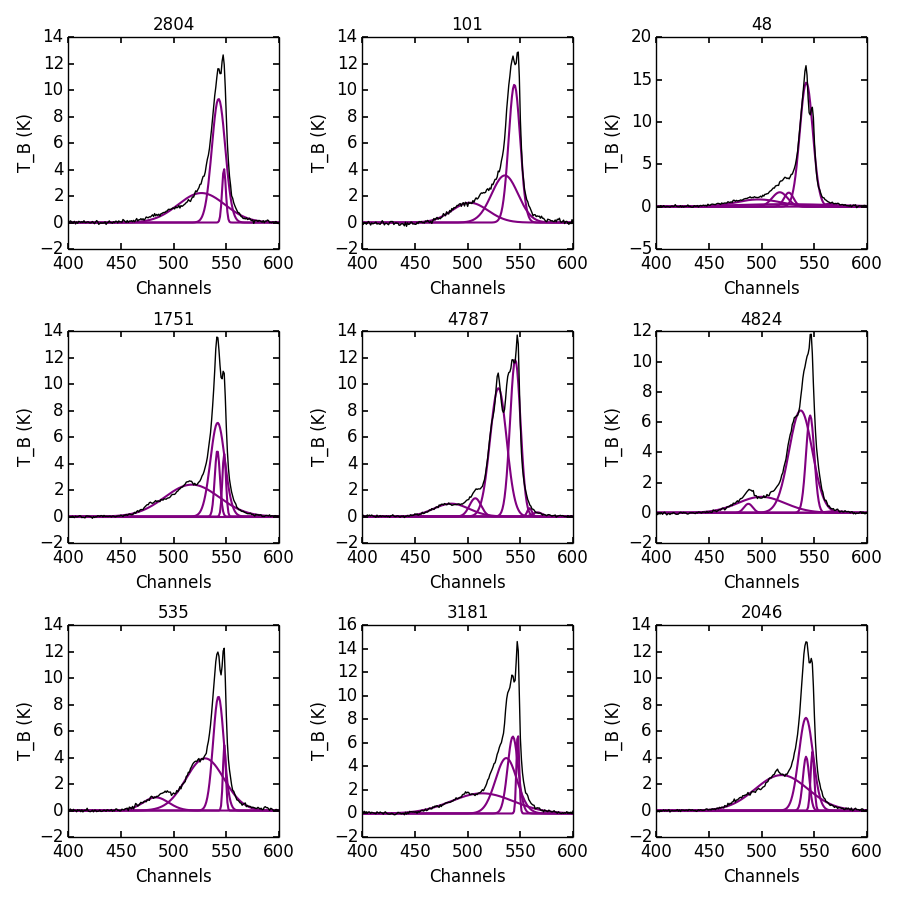
Example spectra from the GALFA-HI M33 datacube, decomposed by GaussPy following two-phase training.

Navigation

Prepping a Datacube¶

Storing Data cube in GaussPy-Friendly Format¶

Creating a Synthetic Training Dataset¶

Training AGD to Select \(\alpha\) values¶

Decomposing the Datacube¶